R for Multivariate analysis
Alternatively see the code at Github
You will need your peak table in a specific format:
- if you have tidied your data using 05_tidy_data_from_MassUp or XCMS, then you should already have the files you need in
"Untargeted_metabolomics_workflow\Tidy_data" - Otherwise you will need a pre-processed peak intensity table saved as a .csv with features (m/z or m/z__RT or m/z bins) as columns and samples as rows in a column called “Sample”. Then you will need either your treatments (classes/ grouping information) in columns following the first column (“Sample”) OR you will need a metadata file with “Sample” as the first column followed by you treatments (classes/ grouping information) in separate columns
Load everything you will need into R
⚠️ you will need to manually install the following packages using
install.packages()or RStudio"tidyr", "tibble", "dplyr", "readr", "stringr", "ggplot2", "pcaMethods", "forcats", "vegan"
Then load all the libraries and functions that you will need by copying this code into R and running it:
source("https://raw.githubusercontent.com/LizzyParkerPannell/Untargeted_metabolomics_workflow/main/00_workflow_functions.R")
Load your data and metadata
Now you can load your peak table. # If you tidied your peak table using our instructions you can use this function to get the peak table.
💡 You need to define MSType as either “XCMS” or “MALDI” (for DI-ESI-MS, use “MALDI”).
peak_table <- get_peak_table(MStype = "XCMS")
And your meta data:
metadata <- get_metadata(MStype = "XCMS")
At this point, it is useful to check how many features are included in your analysis (i.e. how many mz/RT peaks were found). This should be the number of variables in peak_table minus 1 (the 1 being the column of samples). You could report this, for example:
“After grouping and alignment, the processed data comprised XXX features for analysis.”
Run the PCA model
The next step is to arrange the data so that it can be read by the pcaMethods package in R.
The following function will do this and run the initial model.
💡 You need to define MSType as either “XCMS” or “MALDI” (for DI-ESI-MS, use “MALDI”).
results_for_PCA_graphs <- initial_PCA(MStype = "XCMS")
From this we can then make an initial PCA scores plot
# use the function draw_scores_plot to make various graphs (it will automatically tell you the variance associated with the PCs you choose)
# If you only have one class (treatment group) then you still need to define both colour_class and shape_class but they can be the same

scores_plot <- draw_scores_plot(PC_x = "PC1", # these can be changed to PC3, PC4 or PC5
                             PC_y = "PC2", # these can be changed to PC3, PC4 or PC5
                             colour_class = "Time", # choose one of your metadata variables
                             shape_class = "Treat") # choose the same or a different metadata variable

scores_plot

# option to save this plot
ggsave("Tidy_data/PCA_scores_plot.png", scores_plot)
In the above function it is possible to define which combination of principal components you want to show in your 2D scores plot, as well as which classes will be used to colour/shape code your samples.
⚠️ is worth noting that the metadata has not been used in running the model - you are applying the colours after the analysis.
💡 this graph is drawn with
ggplot2so you can use all the functionality of that package to alter the way it looks
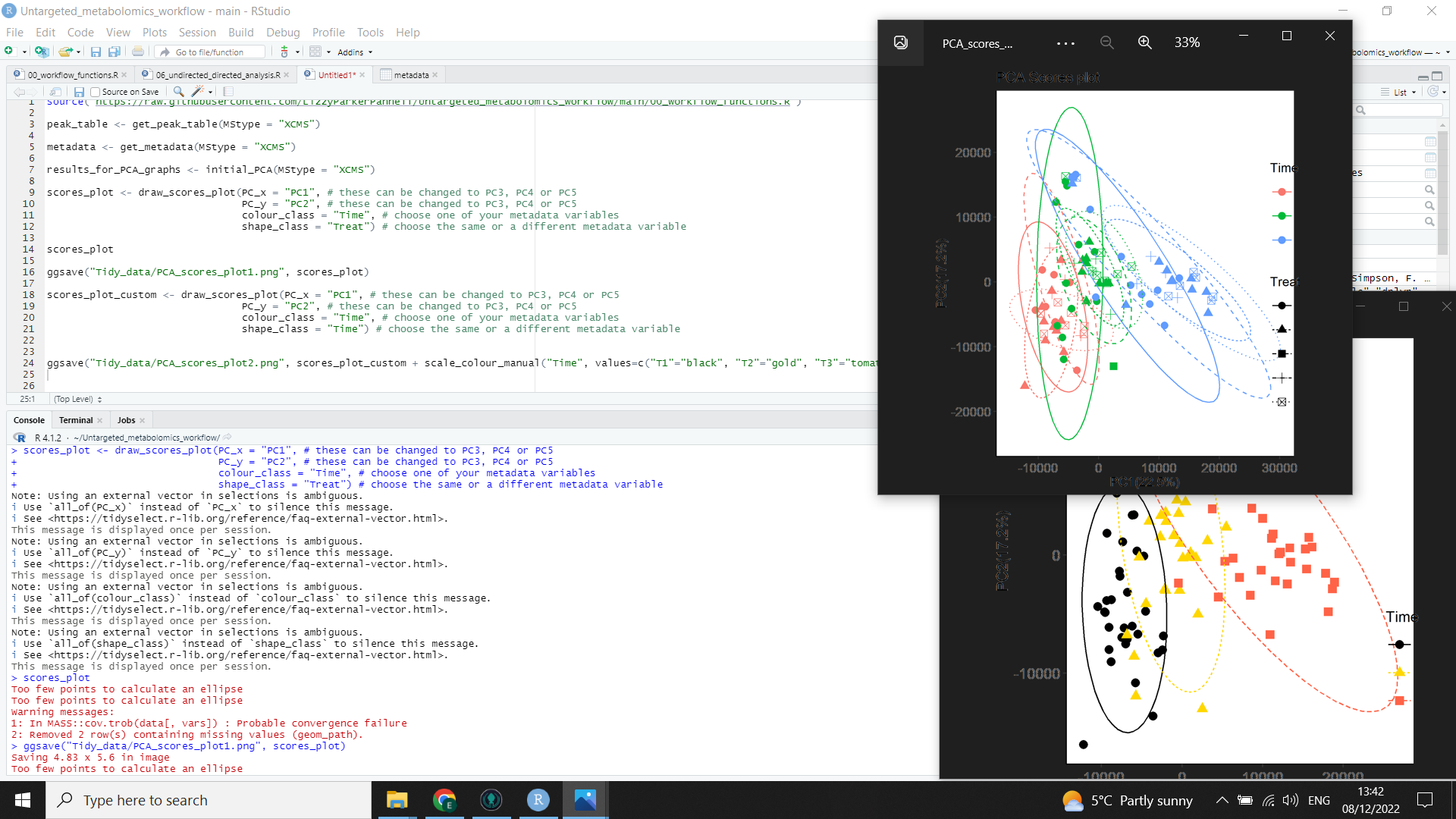
In the above image, you can see the code (left) for both a scores plot (top right) created by the function, and a customised scores plot (bottom right).
Run the PERMANOVA model
A PERMANOVA is another type of multivariate analysis and can help corroborate any differences in your PCA model.
adonis2 from the vegan package is used to run a PERMANOVA.
First we have to do some missing value imputation - you can adjust this if you want to but here we just add 1 (so that there are no zero values) to all intensities
as it is very rare to have an intensity of 1.
impute <- function(x, na.rm=FALSE)(x+1)
permanova_data <- peak_table %>%
select(-Sample) %>%
mutate_all(impute) #if you don't have zeros you will not need to impute
# here you will need to tell the model which metadata you want in your formula:
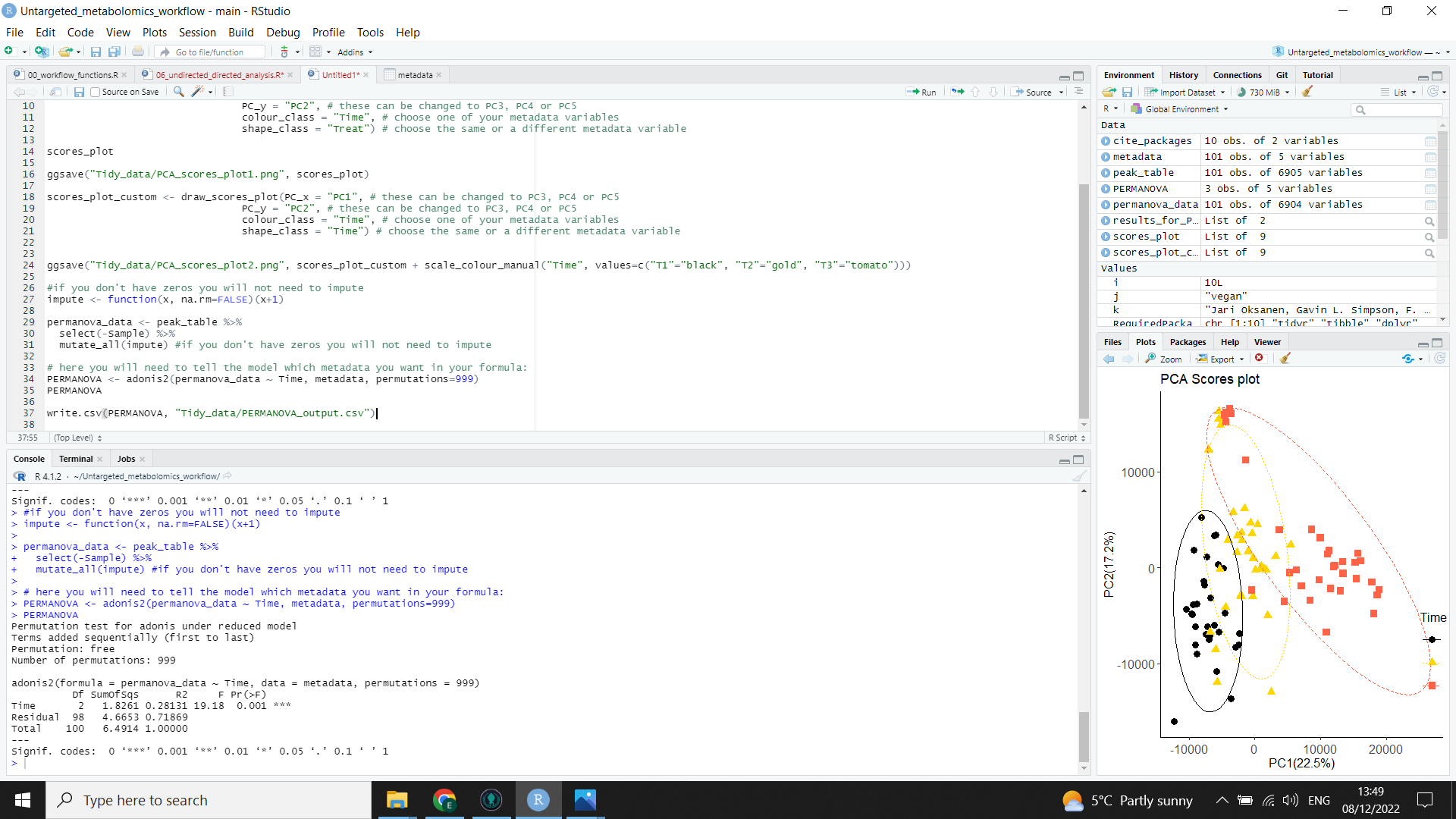
PERMANOVA <- adonis2(permanova_data ~ Time, metadata, permutations=999) # replace "Time" with your class or variable of interest
write.csv(PERMANOVA, "Tidy_data/PERMANOVA_output.csv")
Your result will be saved as a table in the “Tidy_data” folder and displayed in the console as in the image below:
If your groups overlap a lot in the PCA:
Check the following:
- look at scores plots for all combinations of the first 5 PCs
- look through scores coloured by each of your variables
If after this, there is still not much separation between different groups, then there was not a strong difference in metabolomic fingerprint between samples from your different treatment groups using the mass spectrometry approach chosen.
If your groups are different …
If you have some clustering/ separation between your classes then you can use directed analysis to pull out the features (m/z and RT or m/z) that are responsible for the differences between those groups.
… Run the directed analysis (OPLS-DA)
⚠️ The next part of the analysis only works between two groups (called classes from now on). So you need to make some decisions about which groups you need to compare. How you choose to do this will affect the outcome of your analysis so think carefully about what questions you are trying to answer. You could consider:
- sequentially comparing all pairwise combinations of groups
- comparing the two groups which are the most separated in the PCA
- comparing two groups that separate in the PCA where there’s a biological justification for comparison (e.g. from associated experiments on the same biological individuals)
We will use the muma package to run an OPLS-DA (this is a useful guide to OPLS-DA theory).
The next piece of code gets the peak_table (the mz values for each sample) into the format that muma package wants. It will filter the data by the two classes you’re interested in, recode them the way muma wants, and recode your sample names if they are too long (>5. Don’t worry, it will save a file with a key to the new sample names if that’s the case).
# Run the function for the class and levels of that class that you are interested in
tidy_for_muma(metadata_class = "Time",
              class_1 = "T1",
              class_2 = "T3")
Now that the data is in the right format, we can use the muma package as per the documentation.
#here we will use pareto scaling but it is worth exploring whether that is the best scaling for your data
# you will also need to adjust imputation and imput if you have MALDI data (likely to have a lot of missing values)
explore.data(file="muma_undirected_directed_analysis/data_for_muma.csv", scaling="pareto",
scal=TRUE, normalize=TRUE, imputation=FALSE,
imput="ImputType")
# the muma package saves all the output of the analysis to "muma_undirected_directed_analysis/"
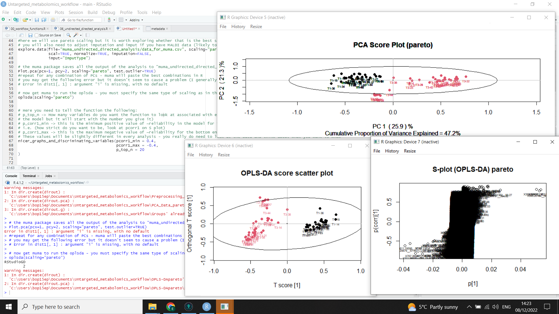
Plot.pca(pcx=1, pcy=2, scaling="pareto", test.outlier=TRUE)
#repeat for any combination of PCs - muma will paste the best combinations in R
# you may get the following error but it doesn't seem to cause a problem (I generally ignore)
# Error in dist1[, 1] : argument "i" is missing, with no default
# now get muma to run the oplsda - you must specify the same type of scaling as in the PCA
oplsda(scaling="pareto")
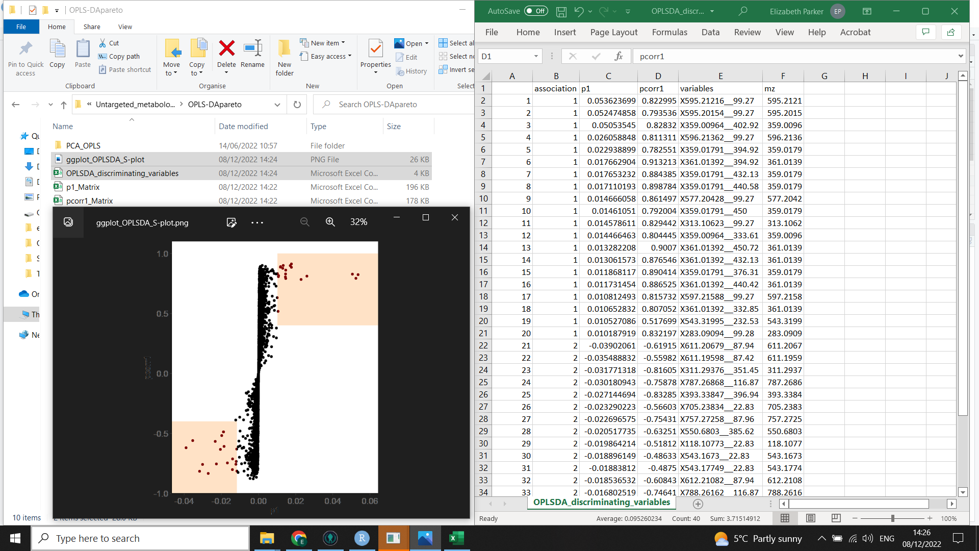
Now we want to produce a list of the most important and reliable variables causing discrimination between the two groups you have compared (which we will need for the next step of the workflow).
This code will also tidy up the S plot created by muma.
⚠️ You will need to play around with this and look at what makes sense for your data. Are you interested in a few m/z values that have a big effect on the metabolomic fingerprint or are you wanting to look at big suites of compounds? Or compounds that are likely to have complex spectra with multiple peaks? You will need to adjust your
p_top_nvalue accordingly.
# Here you need to tell the function the following:
# p_top_n -> How many variables do you want the function to look at associated with each class (you may get fewer returned if they had low reliability in
# the model but it will start with the number you give it)
# p_corr1_min -> this is the minimum positive value of ~reliability in the model for the bottom end of the list of discriminating variables
# i.e. (how strict do you want to be, look at pcorr1 on S plot)
# p_corr1_max -> this is the maximum negative value of ~reliability for the bottom end of the list of discriminating variables
# These values will be slightly different in every analysis - you really do need to look at the data and think about what you want to know

nicer_graphs_and_discriminating_variables(pcorr1_min = 0.4,
                                         pcorr1_max = -0.4,
                                         p_top_n = 20
                                         )
The following image shows the muma output (including PCA scores plot, OPLS-DA scores plot, and S plot)
This second image (below) shows the output from nicer_graphs_and_discriminating_variables() (the list of discriminating variables and a formatted S plot)