Processing DIMS
Pre-processing direct injection ESI-MS data with MassUp
MassUp is open-source software that provides a GUI for processing MALDI-ToF data (or other 2D MS data like our DI-ESI-MS data). It utilises the MALDIquant algorithms but does not require knowledge of R. It also has some nice visualisations (but is a bit old-school to look at. You probably wouldn’t want to use it to make your figures). Here we just use it for quick processing of the data and a bit of quality control.
These instructions are the same as those for processing MALDI data (an dthe example are the same). You may need different parameters but these should be optimised for any experiment anayway.
⚠️ MassUp refers to RAW data a lot but this does NOT mean .RAW files - you need .mzML
📖 The manual and quick start guide are very useful if you want to learn more.
Download MassUp and install on your device
Loading your experimental structure
Open MassUp and click the “import files” icon OR File > Import > Import Files The option of “Labelled” will be automatically selected > OK
Tell MassUp how many treatment groups you have (MassUp calls these “Labels”)
💡 If we have Case vs. Control, we have 2 Labels
Tell MassUp how many samples you have for each Label. You can also rename your Labels at this point (it is possible later too)
💡 If we ran 10 extracts in triplicate for Case and 9 in triplicate for Control, we would have 10 samples for Case and 9 for Control
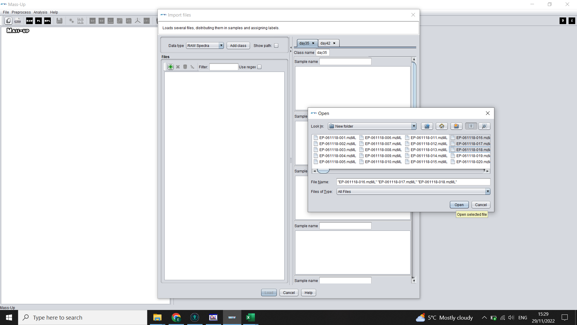
You will now set up the structure of your data. Click on the green plus sign icon and select all the .mzML files from your first treatment group (Label) > OK Highlight these files using shift + left click. Then click on the grey distribute icon. This will distribute these samples in order into the boxes on the left, assuming you have equal numbers of technical replicates and you technical replicates follow on from each other.
💡 If we ran 10 extracts in triplicate for Case, we should select the 30 files that correspond to Case treatment, and will end up with 3 files in each box (Sample)
Repeat for your other labels until you have your complete data structure (MassUp calls this “Labelled data set”)
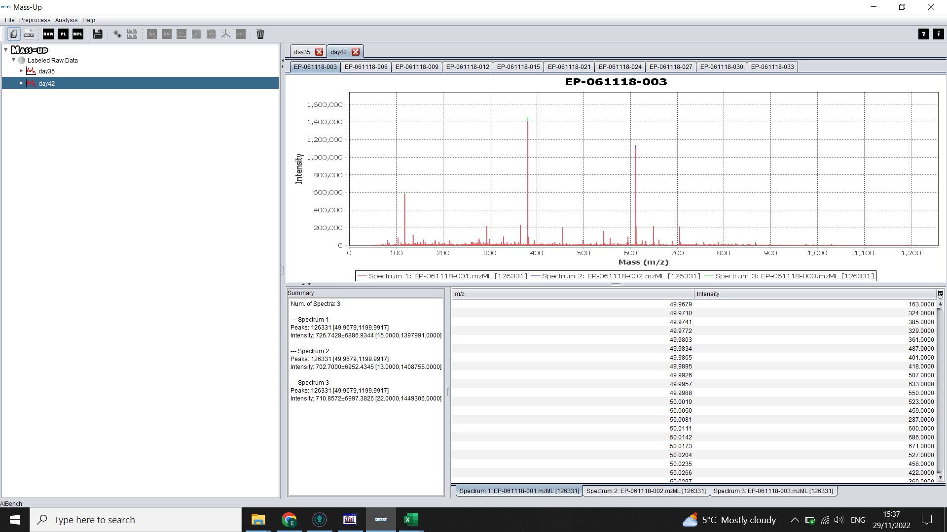
Click “Load” and then when prompted, save your configuration (this saves the labelling, meaning you will be able to load the data more quickly in future). After a couple of minutes, you will be able to look at your raw spectra (the three technical reps will be overlaid in the top right panel). Click through the tabs to see each sample.
Baseline correction , normalization and peak picking
To pre-process the data, click on the icon with two cogs.
Click the double green down arrow icon to select all of your “Labels” (treatment groups)
Use the information in Gibb & Strimmer 2012 1 to decide your settings but select MQ to use MALDIquant, for details on MALDIquant, see the R documentation and manual
Tick the box to “Keep original data”
Click “OK”

You will now have a peak list for each technical replicate.
Alignment (Peak matching)
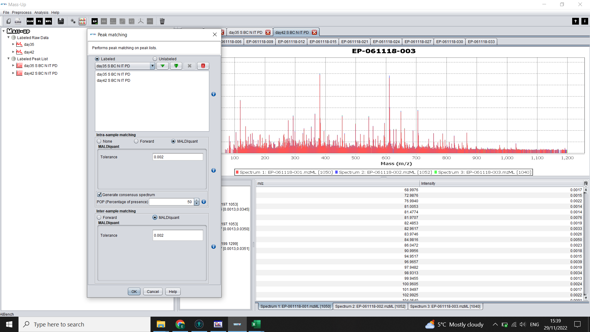
To make consensus spectra (one per biological sample) click on the icon with two graphs (Peak Matching).
Again click on the double green arrow to select both treatment groups (“Labels”).
Select MALDIquant and choose a tolerance level.
Check the box for “Generate consensus spectrum” (you can alter the POP to 100% if you want peaks to be present in all of your technical reps to be considered a peak). Use 50% if any of your technical reps didn’t run properly.
Click “OK”
You will now have an “Inter-matched” peak list for each sample, with samples organised into tabs by treatment group (“Label”)
Basic quality control
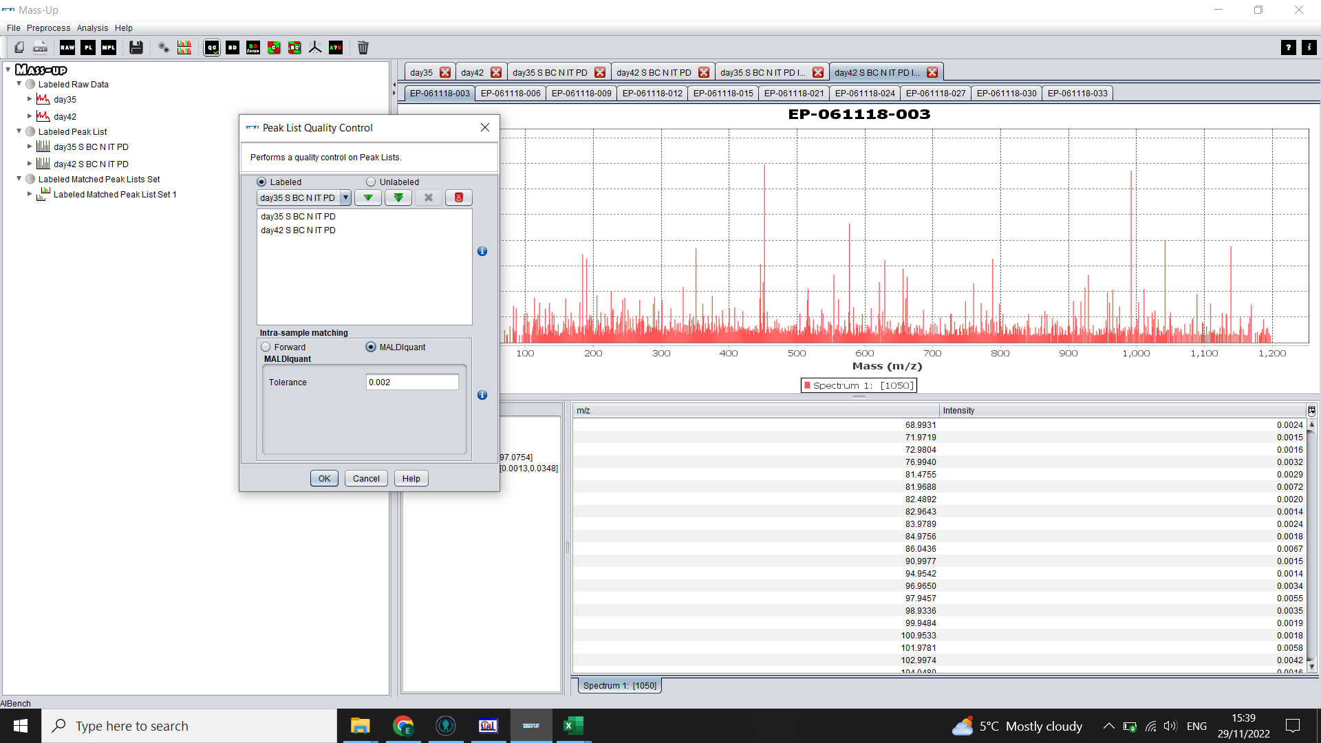
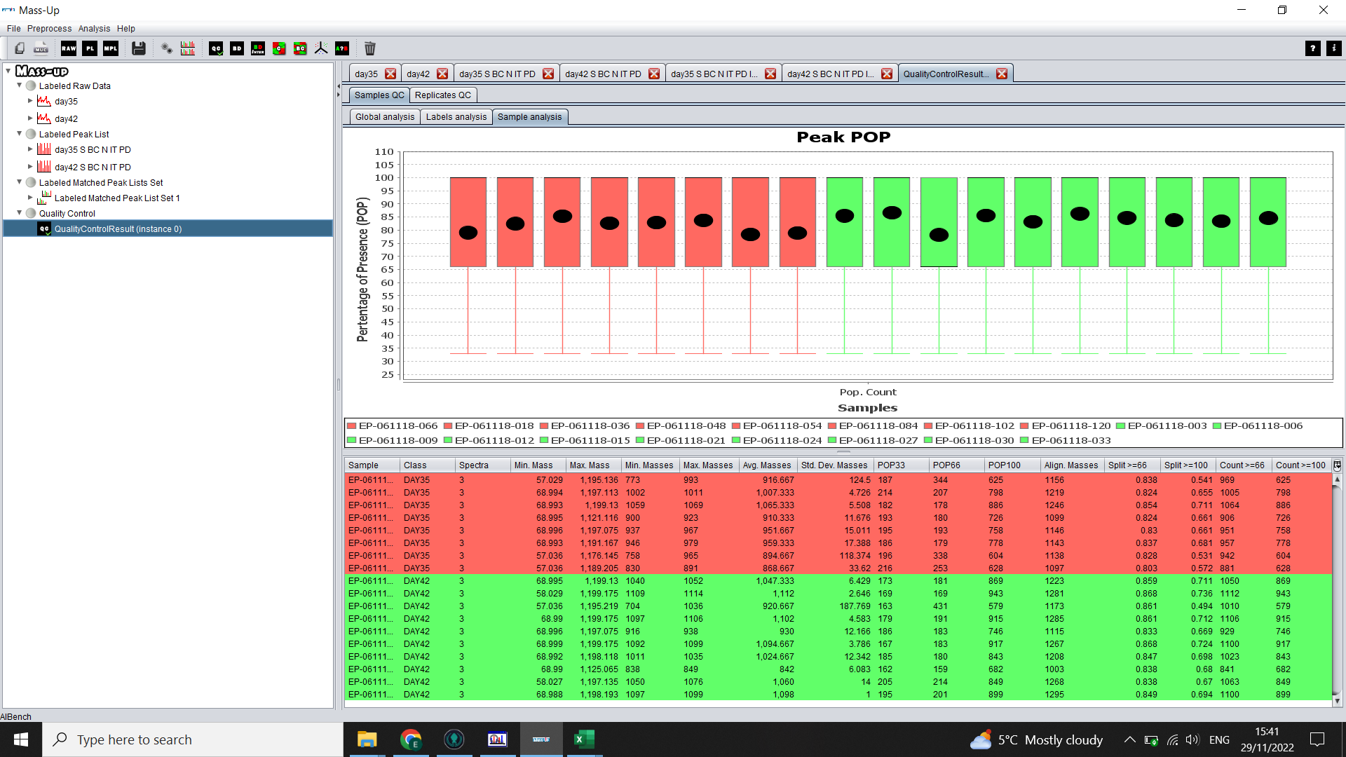
Before further analysis, it is important to take a look at the quality of the data. To do this, click on the QC icon (Quality Control).
Again click on the double green arrow to select both treatment groups (“Labels”).
Select MALDIquant and choose the same tolerance level as above.
Click “OK”.
For more details on the QC, the ? (Help) icon brings up the help/ manual > Operations > The Analysis Menu > Peak List Quality Control
The Replicates QC > Replicates Analysis tab will show a graph with one box per technical replicate and you can compare the percentage of presence of peaks (basically, if there are a few that look very different to the others, you may want to exclude those samples, or at least take it into consideration in your analysis. If there is a lot of variation, you may look into whether there were issues with conversion of the data or with the MS run).
Saving your peak lists
Save your peak lists.
Sadly in MassUp there is no nice way to export a peak table (please let me know if you find one!!!). Instead you have to export each sample’s consensus spectrum and then combine them in R.
Instead we have to export separate .csv files and create our own in R.
To do this, click the “Save” icon in MassUp. Select “Labelled Aligned Peak List” from the dropdown menu, then select the double green arrow to choose all your processed and aligned data. Define an output directory (where you will save your files) and then click “OK”.
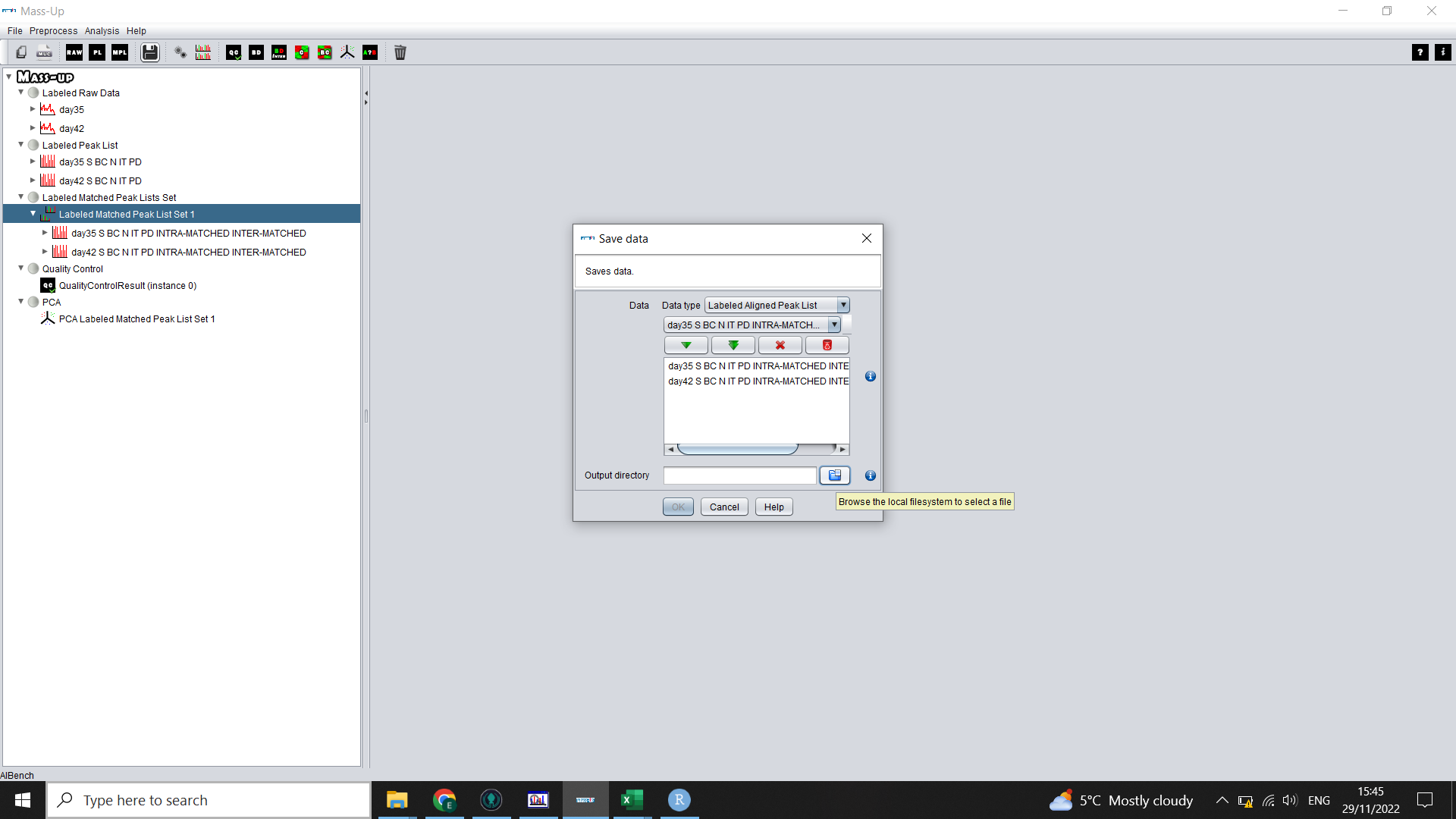
This will save each concensus spectra’s aligned peak list in a separate .csv in quite a frustrating hierarchy of files.
Whilst you will be able to access each spectra .csv from file explorer if you so wish, we will have to do some data tidying in the next step to get a neat peak table for analysis.
-
Sebastian Gibb, Korbinian Strimmer, MALDIquant: a versatile R package for the analysis of mass spectrometry data. Bioinformatics 28(17): 2270–2271 DOI: https://doi.org/10.1093/bioinformatics/bts447 ↩︎